Table Of Content
In many cases, though, the factor levels are simply categories, and the coding of levels is somewhat arbitrary. For example, the levels of an 6-level factor might simply be denoted 1, 2, ..., 6. Physiological measures involve measuring participants’ physiological responses, such as heart rate, blood pressure, or brain activity, using specialized equipment. These measures may be invasive or non-invasive, and may be administered in a laboratory or clinical setting. This involves dividing participants into subgroups or blocks based on specific characteristics, such as age or gender, in order to reduce the risk of confounding variables. This design involves randomly assigning participants to one of two or more treatment groups, with each group receiving one treatment during the first phase of the study and then switching to a different treatment during the second phase.
Understanding Variable Effects in Factorial Designs
This can be seen by noting that the pattern of entries in each A column is the same as the pattern of the first component of "cell". (If necessary, sorting the table on A will show this.) Thus these two vectors belong to the main effect of A. Similarly, the two contrast vectors for B depend only on the level of factor B, namely the second component of "cell", so they belong to the main effect of B. For example, a shrimp aquaculture experiment[9] might have factors temperature at 25° and 35° centigrade, density at 80 or 160 shrimp/40 liters, and salinity at 10%, 25% and 40%.
Don't forget about the “scientist” in your Data Scientist title (Part 2) - Towards Data Science
Don't forget about the “scientist” in your Data Scientist title (Part .
Posted: Thu, 06 Jan 2022 08:00:00 GMT [source]
Lesson 5: Introduction to Factorial Designs
The last four column vectors belong to the A × B interaction, as their entries depend on the values of both factors, and as all four columns are orthogonal to the columns for A and B. Belong to the A × B interaction; interaction is absent (additivity is present) if these expressions equal 0.[13][14] Additivity may be viewed as a kind of parallelism between factors, as illustrated in the Analysis section below. Time series analysis is used to analyze data collected over time in order to identify trends, patterns, or changes in the data. Self-report measures involve asking participants to report their thoughts, feelings, or behaviors using questionnaires, surveys, or interviews.
Main Effects
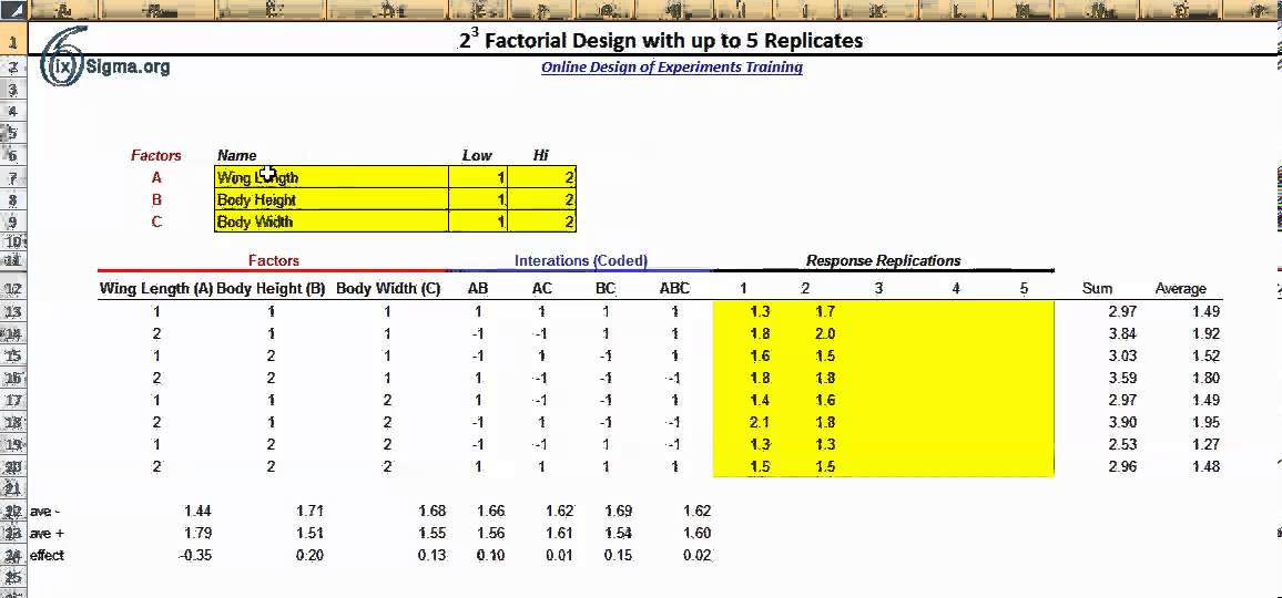
For larger numbers, the factor can be considered extremely important and for smaller numbers, the factor can be considered less important. The sign of the number also has a direct correlation to the effect being positive or negative. If the number of combinations in a full factorial design is too high to be logistically feasible, a fractional factorial design may be done, in which some of the possible combinations (usually at least half) are omitted. Experimental design also allows researchers to generalize their findings to the larger population from which the sample was drawn. By randomly selecting participants and using statistical techniques to analyze the data, researchers can make inferences about the larger population with a high degree of confidence. Experimental research design should be used when a researcher wants to establish a cause-and-effect relationship between variables.
Minitab Example for Centrifugal Contactor Analysis
Moreover, if higher order interactions are not examined in models, researchers will not know if an intervention component is intrinsically weak (or strong) or is meaningfully affected by negative (or positive) interactions with other factors. It is tempting to take advantage of the efficiency of the factorial experiment and use it to evaluate many components since power is unrelated to the number of factors, and therefore, a single experiment can be used to screen many components. However, the number of factors used and the types and number of levels per factor can certainly affect staff burden. A 5-factor design with 2-levels/factor yields some 32 unique combinations of components (Table 1), and requires that at least five different active or “on” ICs be delivered.
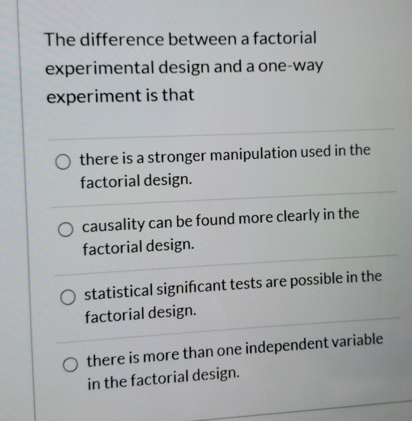
To illustrate a 3 x 3 design has two independent variables, each with three levels, while a 2 x 2 x 2 design has three independent variables, each with two levels. In principle, factorial designs can include any number of independent variables with any number of levels. For example, an experiment could include the type of psychotherapy (cognitive vs. behavioral), the length of the psychotherapy (2 weeks vs. 2 months), and the sex of the psychotherapist (female vs. male). This would be a 2 x 2 x 2 factorial design and would have eight conditions.
That is, one should include only those ICs that are thought to be compatible, not competitive. The choice of control conditions can also affect burden and complexity for both staff and patients. In this regard, “off” conditions (connoting a no-treatment control condition as one level of a factor) have certain advantages. They are relatively easy to implement, they do not add burden to the participants, and they should maximize sensitivity to experimental effects (versus a low-treatment control).
Two-level factorial experiments
Moreover, if instead of “off” or no-treatment conditions, less intensive levels of components are used, then even more ICs must be delivered (albeit some of reduced intensity). In Chapter 1 we briefly described a study conducted by Simone Schnall and her colleagues, in which they found that washing one’s hands leads people to view moral transgressions as less wrong [SBH08]. In a different but related study, Schnall and her colleagues investigated whether feeling physically disgusted causes people to make harsher moral judgments [SHCJ08]. In this experiment, they manipulated participants’ feelings of disgust by testing them in either a clean room or a messy room that contained dirty dishes, an overflowing wastebasket, and a chewed-up pen. They also used a self-report questionnaire to measure the amount of attention that people pay to their own bodily sensations. They also measured some other dependent variables, including participants’ willingness to eat at a new restaurant.
The dependent variable (outcome that is measured) could be how far the car can drive in 1 minute. These independent variables are good examples of variables that are truly independent from one another. For example, shoes with a 1 inch sole will always add 1 inch to a person’s height. This will be true no matter whether they wear a hat or not, and no matter how tall the hat is.
In visually checking the residuals we can see that we have nothing to complain about. There does not seem to be any great deviation in the normal probability plot of the residuals. In the middle - the points in black, they are pretty much in a straight line - they are following a normal distribution. In other words, their expectation or percentile is proportionate to the size of the effect. The ones in red are like outliers and stand away from the ones in the middle and indicate that they are not just random noise but there must be an actual affect. Without making any assumptions about any of these terms this plot is an overall test of the hypothesis based on simply assuming all of the effects are normal.
The result of this study was that the participants high in hypochondriasis were better than those low in hypochondriasis at recalling the health-related words, but they were no better at recalling the non-health-related words. The other was private body consciousness, a variable which the researchers simply measured. Another example is a study by Halle Brown and colleagues in which participants were exposed to several words that they were later asked to recall [BKD+99]. Some were negative, health-related words (e.g., tumor, coronary), and others were not health related (e.g., election, geometry).
One independent variable was disgust, which the researchers manipulated by testing participants in a clean room or a messy room. The other was private body consciousness, a participant variable which the researchers simply measured. Another example is a study by Halle Brown and colleagues in which participants were exposed to several words that they were later asked to recall (Brown, Kosslyn, Delamater, Fama, & Barsky, 1999)[1]. Some were negative health-related words (e.g., tumor, coronary), and others were not health related (e.g., election, geometry). The non-manipulated independent variable was whether participants were high or low in hypochondriasis (excessive concern with ordinary bodily symptoms).
Let's go back to the drill rate example (Ex6-3.MTW | Ex6-3.csv) where we saw the fanning effect in the plot of the residuals. In this example B, C and D were the three main effects and there were two interactions BD and BC. From Minitab we can reproduce the normal probability plot for the full model. The combined main effects are significant as seen in the combined summary table. And the individual terms, B, C, D, BC and BD, are all significant, just as shown on the normal probability plot above. Notice also the use of the Yates notation here that labels the treatment combinations where the high level for each factor is involved.
First, non-manipulated independent variables are usually participant characteristics (private body consciousness, hypochondriasis, self-esteem, and so on), and as such they are, by definition, between-subject factors. For example, people are either low in hypochondriasis or high in hypochondriasis; they cannot be in both of these conditions. Recall that in a simple between-subjects design, each participant is tested in only one condition. In a simple within-subjects design, each participant is tested in all conditions.


No comments:
Post a Comment